In last week’s blog, our research team set out the process of creating a SQLi proof of concept.

Overview

In our previous prototypes we focused on text processing (vectorizing, word2vect, neural networks, etc.). We recognized that despite some signs of potential, the overall approach is difficult because:

It’s not the way the human brain works when detecting vulnerabilities. We don’t read the HTTP response as if we were reading a book. Basically, we try to find specific information within HTTP responses that lets us know what’s happening under the hood. With our existing approaches, we felt that it might not be possible to achieve good results and avoid overfitting at the same time.
Our model(s) will need information for training that doesn’t belong to us. If we could find a way to avoid storing vast amounts of web request/response pairs potentially containing all manner of sensitive information, then this would definitely be a better option.
Our previous prototypes relied on supervised learning, requiring large crowd-sourced pools of our consultants to classify results from actions performed during web application security tests. Despite best intentions, maintaining consistent tagging and supervision in this way could be difficult.

By spending some time on Feature Engineering we were able to explore different models of potential use that would not require client information to be transmitted or stored anywhere outside of our normal Burp installations. We envisaged a system that would implement the feature extraction locally within Burp, and then send only that information to storage for mining and model generation.

In this post we explore an alternative method to identifying potential web application flaws using anomaly detection. One of the main concerns with our other approaches is that a large amount of data is required in order to train the model that, due to its nature, could contain sensitive information – be that client information and/or context-specific sensitive information within web request and response pairs. As a result, we decided to explore an unsupervised learning approach, leveraging large volumes of non-vulnerable URLs to be used in a One-Class or clustering approach. In essence, we changed the problem by training a model of ‘known good’ so as to identify anomalies of ‘possible bad’, as opposed to training a model of ‘known bad’ so as to spot future ‘potential bad’.

Common Crawl

Common Crawl [1] is a non-profit organization that crawls the web and freely provides its archives and datasets to the public. Common Crawl’s web archive consists of petabytes of data collected since 2011. It completes crawls generally every month.

For our research, the January 2019 file was downloaded, and a dataset of URLs was created. The initial idea was to run a scan against this set of URLs. Assuming that they (or at least most of them) are not vulnerable, we thought that it would be possible to train models that could recognise non-vulnerable apps and, as a result, identify any vulnerable sites that do not fit with what we consider a non-vulnerable app.

However, the Common Crawl dataset includes all kinds of websites. Scanning most of them without previous authorization would be in breach of various global legislation on computer misuse. As such we abandoned this avenue of research.

Bug bounty Programmes

The best option identified to avoid the issues described above was to run our scans and create two datasets based on URLs included in bug bounty programmes such as HackerOne [2].

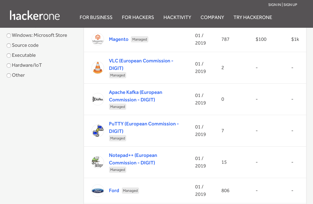
Figure 1 – HackerOne Bug Bounty Programme

It was found that using URLs from these open bounty targets would avoid legal problems so long as we didn’t induce any Denial of Service conditions. Also, since the assets in scope are usually mature in terms of security, most of automated scans we would run (or even all of them) would not likely find a vulnerability, allowing us to assume that certain URLs belong to the class of “not vulnerable” in our experiments.

A GitHub repository containing a list of eligible domains for bug bounty programmes hosted by HackerOne and Bugcrowd [3] was found to be useful to filter the domains that could be included in our dataset.

Logger++ Burp Extension

Once we had a set of URLs to test against, it was necessary to find a way to extract all information associated with each connection to be used in our experiments.

The first approach was to use the Logger++ Extension [4] for Burp Pro, developed by NCC Group and one of the most used public extensions in the BApp Store. This extension allowed us to register information for each connection generated by Burp Intruder and store this in CSV format, or to send the data to our internal elasticsearch service. However, it was found that the “export to ElasticSearch” feature did not include the full request and response, thus the source code was forked [5] from GitHub and an additional option was added that allowed us to include all request and response information within our internal elasticsearch instance. This new feature has been contributed as a Pull Request [6] to the master codebase.

The extension logs the following information:

host
method
newcookies
path
protocol
referrer
requestbody
requestcontenttype
requestlength
requesttime
responsebody
responsedelay
responselength
responsetime
sentcookies
status
title

Since the information did not include the specific payload that was tested, a custom HTTP header “X-Check” was created. This header included the payload in use on each request, so it could be logged as a part of the request body.

Feature Engineering

After a study of the information available, a number of features were extracted from the data collected. Some of those features were based on the responses of each request, whereas others were based on the difference between the response to a request and the response of what we called the reference request, which is the request that Burp Intruder performs first (request 0) without any specific payload:

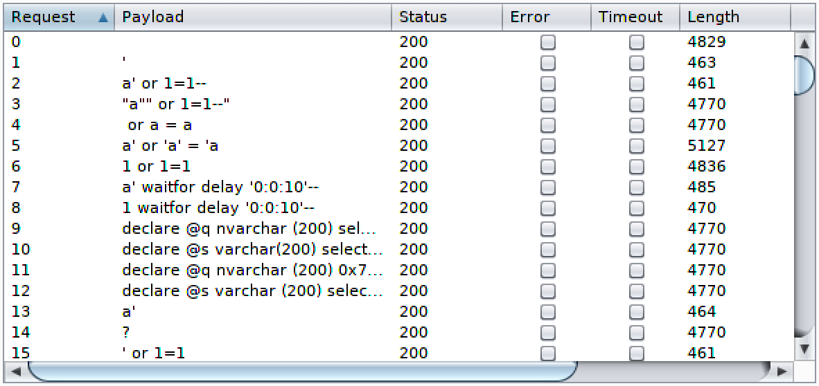
The features selected are shown below:

Status: HTTP Response code, in a numeric format (200, 302, 404, etc).
Status Encoded: Since using a numeric value for “status” would result in strange results (“200” code would be more similar to “302” than to “404”, which is not true), a One Hot Encoding approach was used. 10 features were created based on the “status” code, encoding each group of HTTP response codes in a different way. A few examples are shown below:

	1xx	2xx	3xx	4xx	5xx
200	0	0	1	0	0	0	0	0	0	0
302	0	0	0	0	1	2	0	0	0	0
404	0	0	0	0	0	0	1	4	0	0

Status Difference: Difference between the status code of the reference request and the current request.
Response Size: Number of bytes in the response of the current request.
Response Size Difference: Difference between the number of bytes in the response and the reference request, and in the current request.
Number of lines in Response: Amount of lines in the response of the current request.
Difference of lines in Response: Difference between the amount of lines in the response in the reference request and in the current request.
Length of largest line in Response: Length of the longest line found in the response of the current request.
Difference in the largest line in Response: Difference between the length of the longest line found in the response in the reference request and in the current request.
Mean length of lines in Response: Mean of line lengths in the response of the current request.
Difference in the mean length of lines in Response: Difference in the mean of line lengths in the response of the reference request and of the current request.
Response Delay: Delay in milliseconds between request and response of the current request.
Difference in Response Delay: Difference in milliseconds between response delay of the reference request and the current request.
Response Body Statistics: Number of vowels, consonants, numbers, whitespaces and symbols (5 features) per response length.
Difference in Response Body Statistics: Difference between the number of vowels, consonants, numbers, whitespaces and symbols (five features) per response length in the response of the reference request and of the current request.
Body Difference Statistics: Number of vowels, consonants, numbers, whitespaces and symbols (5 features) per length of the text difference (diff) between the response of the reference request and the response of the current request.

A python script [7] was created that connected to the internal elasticsearch service, obtained all information and exported all the features described above in CSV format.

Data normalisation

Normalisation is a term used in statistics that means to adjust values measured on different scales to a common scale such as [0, 1] or [-1, 1]. Data normalisation is necessary in many Machine Learning models, since a feature with much wider values range would have more weight in the final decision than other features.

Based on the options implemented in “sklearn.preprocessing” [8] the following alternatives were evaluated:

Scale [9]: Standardise features by removing the mean and scaling to unit variance. Since this normalisation is based on the mean, it was affected by extreme values. A very big or very small value would affect the mean and, as a result, all values in the new scale.
MinMaxScaler [10]: Transform features by scaling each feature to a given range, usually [0, 1]. However, the same happened as with the “Scale” normalisation, and extreme values affected the resulting scale, since all values were distributed in that range proportionally.
RobustScaler [11]: Standardise features by removing the median and scaling according to the quantile range, usually the IQR (range between the 1st and 3rd quantile). Since this scaler is based on the median, it is much more resistant to extreme values than the scalers mentioned above.

After some tests, it was found that the “RobustScaler” provided the best normalisation for our particular problem. This was because our datasets may or may not include samples belonging to a second class, usually known as “outliers”. Those outliers are usually extreme values that do not fit to the same model that most of the values fit. Because of the reasons explained above, the RobustScaler is specifically designed to manage those values and normalise the values in a way that is useful for further outlier detection.

*Figure 3 – Values (:27) after RobustScaler normalisation*

Unsupervised learning models

Unsupervised machine learning algorithms infer patterns from a dataset without reference to known, or labelled, outcomes [12]. This approach is particularly useful when a dataset of classified samples is not available, or involves a high cost to generate.

One of the most extended applications of unsupervised learning is clustering. A clustering approach tries to group samples that are similar to each other, creating potential classes.

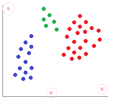
*Figure 4 – Clustering and outlier detection*

Those samples that are not grouped together with one of the classes are called outliers. This concept is used in anomaly detection, where we have a dataset of unclassified data belonging to what we consider a “normal behaviour” and we want to find anomalies and predict problems.

When it can be guaranteed that our training dataset does not contain outliers, it is called Novelty Detection. When we may have some outliers (also known as “contamination”) in the training dataset, it is called Outlier Detection [13].

Our research focused on outlier detection. When scanning a specific website, we assume that most of the checks that are performed will not find any vulnerability. Those checks can be modelled using a number of clusters. An outlier detection on this dataset should result in detecting those checks that created an anomaly response, which should mean an issue is detected.

Data analysis

As described above, after normalisation we analysed each feature in a separate way to check what kind of distribution they followed. The result of creating a histogram for each feature is shown below:

*Figure 5 – Distribution of each feature given a specific web application login dataset*

Gaussian Mixture

A Gaussian Mixture [14] Model (GMM) is a probabilistic model that assumes all data points are generated from a mixture of a finite number of Gaussian distributions with unknown parameters.

The first stage of this approach is to find how many Gaussians are necessary to fit a given dataset. The Bayesian Information Criterion (BIC) and the Akaike Information Criterion (AIC) is a measure of how well a GMM fits a specific dataset. Both criterions introduce a penalty term for the number of gaussians used in the model, since obviously a dataset of 100 samples could perfectly be generated by a GMM of 100 Gaussians. This problem is called “overfitting” [15] and represents one of the biggest challenges in data science.

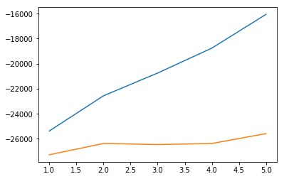
*Figure 6 – BIC (blue) and AIC (orange) per number of gaussians*

It was found that AIC was particularly good for outlier detection. BIC includes a bigger penalty than AIC when the number of Gaussians are increased, which means that the model with the best BIC was always based on a single Gaussian estimator, with a higher probability of detecting regular samples as outliers. Because of this, it was decided to use the number of estimators that were found to result in the lowest AIC score.

The model with the lowers AIC score was selected and the score (likelihood) for each sample of the dataset calculated. A histogram of those values is shown below:

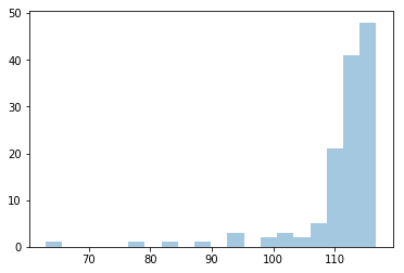
In this specific circumstance, we know that all samples in the dataset are (assumed) non-vulnerable detections, but we see that a few values were scored under 70, which is much less than the rest of the scores.

As a first approach, an empiric threshold was created:

Outlier if score > 200: A very high score means that an estimator was used only for this sample, and no other close samples affected its mean and standard deviation.
Outlier if score < 2*median – max: Formula derived from IQR.
Inlier otherwise.

As a result, we obtained an empty list of outliers, which fits with the dataset.

(array([], dtype=int64), array([], dtype=int64))

A second experiment was conducted. Three artificial outliers were introduced by mutating regular samples, creating new samples with more extreme values than the regular samples. It was necessary to recalculate from the beginning how many estimators we need to fit this new dataset.

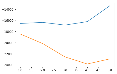
*Figure 8 – BIC (blue) and AIC (orange) per number of gaussians*

It was found that, after including the three artificial outliers, the AIC score was significantly better when using 4 estimators.

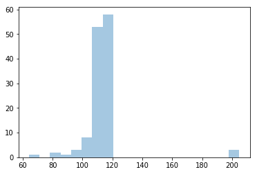
*Figure 9 – GMM scores with three outliers*

A histogram of the scores revealed that some samples had a really big score, corresponding to samples where the model used a specific estimator for that sample. If we use the same threshold mechanism mentioned above, we find that our model detected the three outliers that were introduced in this experiment.

(array([], dtype=int64), array([126, 127, 128]))

We can observe that the non-vulnerable samples were estimated from a single Gaussian, whereas the other three Gaussians estimated one outlier each.

Local Outlier Factor

The Local Outlier Factor (LOF) technique [16] measures the local deviation of density of a given sample with respect to its neighbours. The local density of a given object is calculated based on the distance to the k-nearest neighbours (KNN). Those objects with a substantially lower density are considered outliers. First, we performed an experiment that obtained the number of outliers detected given a number of neighbours to be considered:

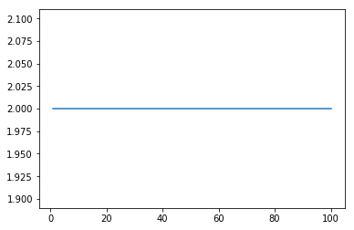
*Figure 10 – Outliers / neighbours considered*

It was found that this model always found two outliers independently to the number of neighbours being considered. However, we know that this dataset does not contain any outlier, so it was not obtaining accurate results anyway. A second experiment was conducted by using a static number of neighbours (10) and different contamination rate, from 0.00001 to 0.1. The contamination rate is the rate of outliers that are expected in our dataset.

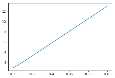
*Figure 11 – Outliers / Contamination Rate*

The model adjusts the number of outliers detected based on the contamination rate. Because of this, the model will always find more outliers if we parametrise a bigger contamination rate, even when the dataset does not actually contain outliers. The following two outliers were found in the experiment described above:

(array([ 6, 86]),)

Because of this, when we created three artificial outliers and we repeated the same experiments, we obtained the same results, but the two outliers detected were two of the three samples generated, and the remaining sample was not identified including any as outliers:

(array([126, 127]),)

Isolation Forest

An Isolation Forest [17] is similar to Random Forest but specially designed to be used in anomaly detection problems. When creating a tree, a feature is randomly selected, and a random split of the space is created. The number of splits required to isolate a sample is a measure of how isolated this sample is. Outliers should have a low score, since they are more easily isolated when performing a random split than Inliers.

*Figure 12 – Outliers / Contamination Rate*

An experiment was conducted by trying different contamination rates, from 0.00001 to 0.1 with a fixed number of estimators (5). As witnessed in previous experiments, the contamination rate directly impacted on the number of outliers detected. We selected a contamination rate of 0.001 for further experiments.

Using this parametrisation, we detected an outlier in a dataset where no outlier was present. In a second experiment we introduced three artificial outliers, but the model detected the same outlier as in the previous experiment.

 (array([86]),)

Elliptic Envelope

Elliptic Envelope [18] tries to define the “shape” of the data by fitting a robust covariance estimate to the data, and thus fits an ellipse to the central data points, ignoring points outside of the central mode.
The same experiment described above was repeated for this model. A set of contamination rates were tested, obtaining the number of outliers detected when using each of them.

*Figure 13 – Outliers / Contamination Rate*

The model adjusts the number of outliers detected based on the contamination rate. Because of this, the model will always find more outliers if we parametrise a bigger contamination rate, even when the dataset does not actually contain outliers. The following two outliers were found in the experiment described above:

 (array([86, 93]),)

Because of this, when we created three artificial outliers and we repeated the same experiments, we obtained the same results, but the two outliers detected were two of the three samples generated, yet the remaining sample was not identified as outliers.

 (array([126, 127]),)

One-Class SVM

One-Class SVM [19] is a particular kind of Support Vector Machine (SVM) where the hyperplane used as a decision border has been substituted by a hypersphere. The main goal of One-Class SVM is to find the hypersphere with minimum radio that contains all the dataset.

Since the samples only have a spherical shape in certain situations, SVM typically uses a previous transformation of the space (kernel). A good kernel selection strongly impacts on the results, since the resulting space could fit much easily to a hypersphere shape.

Our first experiment was to use all the available kernels with default parametrisation on a dataset where only non-vulnerable samples were present. For each of them, the number of outliers detected was obtained.

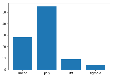
*Figure 14 – Number of Outliers using each Kernel*

Further testing revealed that, in general, “rbf” kernel had better results than “sigmoid” kernel, despite the fact that with default parametrisation, the “sigmoid” kernel detected fewer outliers in a dataset where we shouldn’t have found any outlier.

Our second experiment was to use an “rbf” kernel and iterate values for the “gamma” parameter. The “gamma” parameter is the Kernel Coefficient, so it impacts in a different way depending on the Kernel in use.

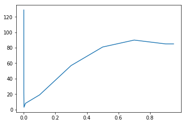
A “gamma” value of 0.001 was found to result in the smaller detection of outliers, which is the desirable behaviour in this dataset.

Finally, we iterated several values of the contamination rate, as we did in previous experiments.

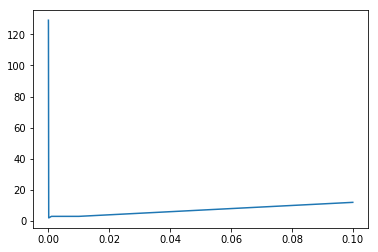
A contamination rate of 0.0001 was found to be the best parametrisation to fit our dataset. However, two samples were wrongly detected as outliers.

(array([41, 57]),)

When introducing three artificial outliers, it was found that this model detected three outliers, but one of them (86) was not one of the outliers introduced in the dataset.

 (array([ 86, 127, 128]),)

Conclusions

From our experiments, it was found that most Outlier Detection mechanisms explored in this research required a previous knowledge about the rate of outliers we expect (the “contamination” rate). When this rate is completely unknown, as happened in our specific problem, it is difficult to find a rate that fits our dataset when there aren’t outliers included and that, at the same time, detect outliers when they exist in our datasets.

Because of these results, we selected a Gaussian Mixture Model (GMM) to be used in a complete proof of concept, since it was the only one not strongly tied to a contamination rate.

As a last experiment, we reproduced the previous experiments using a different dataset, obtained from Burp Intruder data gained from trying to find SQL Injection vulnerabilities in the Damn Vulnerable Web App Docker container, which is obviously vulnerable to SQL Injection.

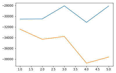
*Figure 17 – BIC (blue) and AIC (orange) per number of gaussians*

An AIC comparison revealed that this dataset could be fit by using 4 estimators (Gaussians), resulting in the following score histogram:

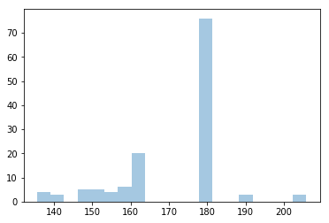
The outliers were detected based on their scores and the algorithm that we described in previous sections:

(array([ 0, 12, 25, 27, 29, 30, 44, 49, 56, 70, 78, 80, 86,
 90, 91, 92, 93, 96, 100, 105, 115, 128]), array([ 9, 50, 82]))

This result was expected, since several of the payloads used in this experiment resulted in SQL errors shown in the webpage. It confirms that our Outlier Detection approach could be valid and produce good results in real-world applications.

Burp Extension PoC

A Burp Extension was developed in python as a proof of concept – however Burp Extensions are executed using Jython, so libraries relying on C code such as sklearn couldn’t be used. Because of this, we separated the functionality into two different parts:

ava.py: this is the Burp extension that collects the information, extracts the features and requests the HTTP API for a classification
avasrv.py: exposes an API that is used by ava.py to upload the dataset and obtain the outliers

ava.py was supposed to add a note in the Burp Intruder column “Notes” or to colourise the row, however a bug in Burp Suite restricted such implementation. The bug was reported to PortSwigger and it will be fixed in the next release – until such time, our extension prints the outliers in the standard output for testing purposes.

References

Written by NCC Group
First published on 20/06/19

Matt Lewis

Jose Selvi

Project Ava: On the Matter of Using Machine Learning for Web Application Security Testing – Part 7: Development of Prototype #3 – Adventures in Anomaly Detection