Written by Jose Selvi and Thomas Atkinson
If you are a Machine Learning (ML) enthusiast like us, you may recall our blogpost series from 2019 regarding Project Ava, which documented our experiments in using ML techniques to automate web application security testing tasks. In February 2020 we set out to build on Project Ava with Project Bishop, which was to specifically look at use of ML techniques for intelligent web crawling. This research was performed by Thomas Atkinson, Matt Lewis and Jose Selvi.
In this blogpost we share some of the preliminary experiments that we performed under Project Bishop, and their results, which may be of interest and use to other researchers in this field.
The main question we sought to answer through our research was whether a ML model could be generated that would provide contextual understanding of different web pages and their functions (e.g., login page, generic web form submission, profile/image upload etc.). The reason for this focus was that we learned under Project Ava, that human-based interaction would first be needed to identify the role/function of a web page, before it could then initiate the appropriate ML-based web application security test (e.g., SQLi, XSS, file upload etc.). Intelligent crawling would minimise the requirement for human interaction and thus maximise the potential level of automation in ML-based web application security testing.
In order to obtain data for use in our experiments, we obtained the popular Alexa Top 1K (Note: this service has since been retired), which is a list of the most visited websites on the Internet. The initial plan was to obtain information about the main page of each of these websites and to classify them. However, this dataset included URLs, but not the nature or purpose of each one of those websites. For this reason, we decided to focus on finding a good representation of their content and using clustering techniques to find which websites looked most alike.
We created a python tool, which relied on Selenium to visit each one of the target websites and obtain the information that was used later to feed our ML models.
In particular, the following information was obtained:
- Source Code: We used the Selenium’s “page_source” feature to obtain the source code of the websites. This was stored in a HTML file.
sauce = browser.page_source - Screenshot: We used the Selenium’s “save_screenshot” feature to obtain a screenshot of the website. This was stored in a PNG image.
selfie = browser.save_screenshot(name + ".png") - Visual Page Segmentation (VIPS): We used wushuartgaro’s python implementation of the Microsoft Visual Page Segmentation (VIPS) algorithm. This was stored in a JSON data structure, which includes information about how the HTML elements are displayed.
file = open("dom.js", 'r')
jscript = file.read()
jscript += 'nreturn JSON.stringify( toJSON( document.getElementsByTagName("BODY")[0] ) );'
jason = browser.execute_script(jscript)
The VIPS JSON format includes additional information such as the position and size of each one of the elements in the body, among other characteristics describing how each one of these elements were visualized when they were rendered. An example of this format can be observed bellow:
{
    "nodeType": 1,
    "tagName": "a",
    "visual_cues": {
        "bounds": {
            "x": 118,
            "y": 33,
            "width": 80.265625,
            "height": 11,
            "top": 33,
            "right": 198.265625,
            "bottom": 44,
            "left": 118
        },
        "font-size": "11px",
        "font-weight": "700",
        "background-color": "rgba(0, 0, 0, 0)",
        "display": "block",
        "visibility": "visible",
        "text": "Iscriviti a Prime",
        "className": "nav-sprite nav-logo-tagline nav-prime-try"
    },
Finally, we combined this output to create our initial dataset, based on the Alexa Top 1K information.
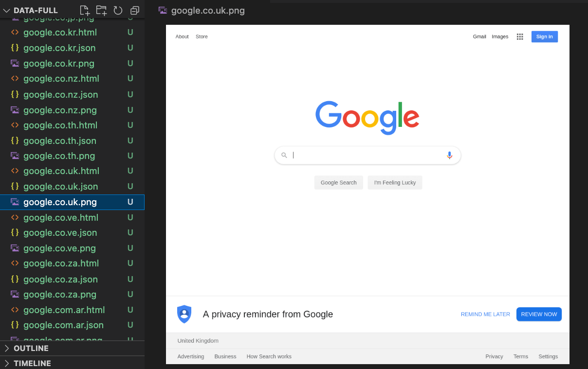
Figure 1 – Dataset including HTML, PNG and JSON files for each website
Simple Feature Extraction with Unsupervised Convolutional Neural Network (CNN)
One of the re-occurring themes from our background research in Project Bishop was the use of CNNs for feature segmentation. This technique showed potential promise if applied to the screenshots of web pages that we had gathered previously. We experimented with CNNs, using the models developed by Asako Kanezaki presented in her 2018 paper “Unsupervised image segmentation by backpropagation”. This approach used a simple unsupervised CNN to automatically extract features from images. Kanezaki found good results when applying this technique to images with large objects like cars, bears, people etc. Some limitations were however observed regarding the style and imagery of some web pages. Below are examples of an input image and output result:

Figure 2 – Input web page image
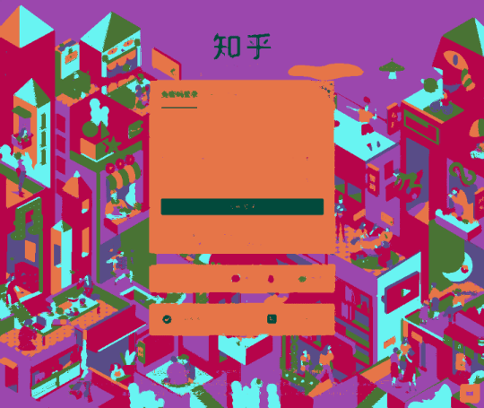
Figure 3 – Difficulties with feature extraction on busy/dense backgrounds
As shown in Figure 3, the model focused mainly on large blocks of solid colours and many of the features and finer details required for browsing were lost. This example is a good one as the input data has a particularly busy background that a human can automatically recognise as a background image.
This experiment showed that a simplistic approach such as this focused on too high a level and was also not fit for extracting subtle yet important features.
Manual Feature Extraction from JSON
We tried to manually extract several features from the information that we had (HTML, DOM, JSON, screenshot-png). From state of the art as seen from our Internet searches, we couldn’t find a reference of features that yielded good results when trying to solve similar problems. Most of the classification problems that we found were based on the textual information contained in the page, which can be used to determine if a page is related to a category such as sports, philosophy or technology. However, the problem we were trying to solve was far different and therefore, those techniques and features were not useful to our research.
As a first approach we focused on the DOM, since the HTML could not contain all the information necessary to represent the rendered page. In particular, the HTML content could not be enough to represent single-page applications, since the same HTML content could result in different rendered pages depending on further connections.
In our first experiment we used the following features extracted from the DOM:
- # input elements
- # buttons
- # images
- # links
- # texts
Using these features, we used the K-Means techniques to cluster together all pages that could look similar or have similar behaviour based on the features we extracted. For our experiment, we established a fixed amount of 10 clusters:
| CLUSTER | # ELEMENTS | EXAMPLES |
| 0 | 730 | duckduckgo.com ebay.co.uk |
| 1 | 1 | kijiji.ca |
| 2 | 1 | globo.com |
| 3 | 2 | att.com eventbrite.com |
| 4 | 2 | instructure.com zendesk.com |
| 5 | 1 | webmd.com |
| 6 | 1 | kickstarter.com |
| 7 | 1 | playstation.com |
| 8 | 3 | reddit.com rt.com |
| 9 | 8 | expedia.com msn.com |
These results did not look to fit what we see in the real world, which showed that the features that we were using were not a good representation of the pages.
To increase the number of features, we included the features that provided a sense of position, based on the distance from each element to the centre of the page, or from the bottom left to the element. We repeated the same experiment with K-Means clustering with these new features, but the results were similar to our previous attempt.
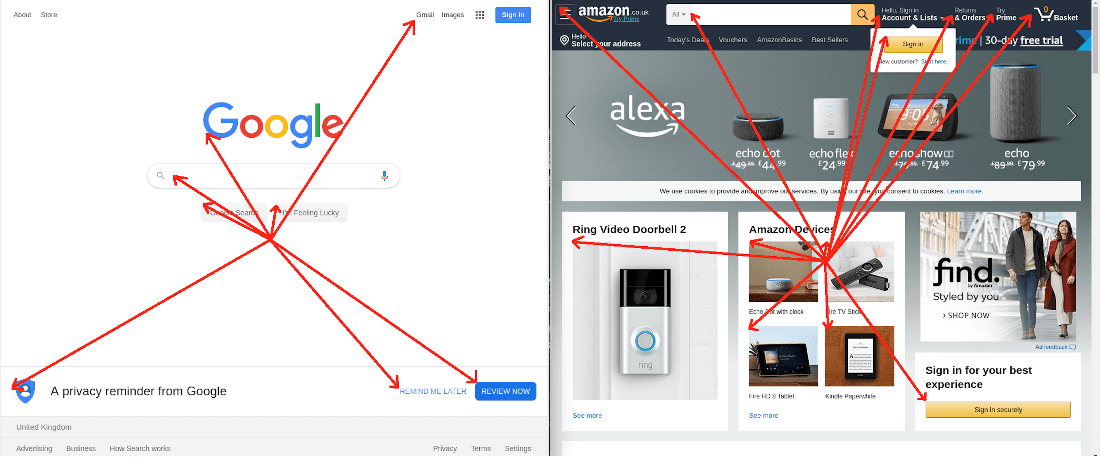
Figure 4 – Using a feature based distance from each element to the centre of the page
We realised that feature extraction from a web page is a difficult problem that cannot be solved by using a simple approach such as the one described above. We decided to then explore other techniques such as automatic feature extraction based on the screenshots that we could generate by rendering the DOM.
First, we created a secondary representation of the screenshot. This approach was borrowed from the field of autonomous driving, where a technique called “semantic segmentation” refers to the process of linking each pixel in an image to a class label. These labels could include a person, car, flower, piece of furniture, etc., just to mention a few. This representation removes certain information, such as textures, that are not relevant for further decisions, so it allows for a simpler and more efficient training processes.
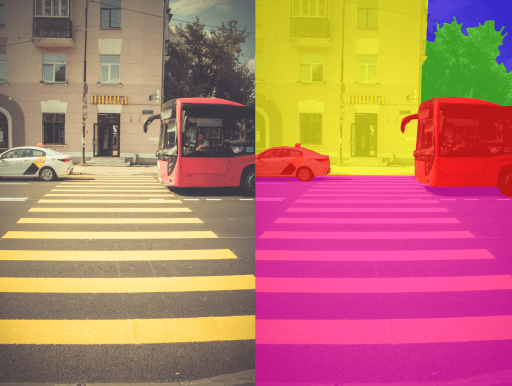
Figure 5 – Semantic Segmentation in Autonomous Driving (reference)
Recall from earlier that our dataset included information extracted using a well-known heuristic technique called “Vision-based Page Segmentation Algorithm” (VIPS) published by Microsoft. In particular, we used a Python implementation called “VipsPython” available on GitHub, with a few small modifications.
To obtain our semantic representation, we created a small python script that explored the structure of the JSON file and created a new image by drawing on it each one of the elements of interest, using different colours for different elements, as follows:
- Images: Green
- Input Elements: Red
- Buttons: Blue
- Links: Black
The image bellow shows the original website (facebook.com) and its corresponding semantic segmented image, using this technique. This new image keeps the information about where visual elements of the website are located, but it removes other additional information such as a specific image, textures, texts, etc. This may help our models to focus on what is important in the image.
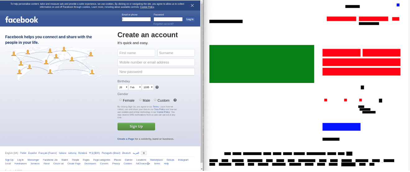
Figure 6 – Facebook.com and its semantic segmentation representation
In terms of models to be used, neural networks usually provide good results when handling visual representations such as images. However, for unclassified datasets (unsupervised learning), neural networks are not easy to use, since the back-propagation algorithm requires the result of the classification to be compared with the expected result to re-calculate the weights of the interconnections between neurons. Since our dataset was not classified in any way, a regular approach based on neural networks was not possible.
To avoid these problems, we used a specific design of neural network called Autoencoder, which has been used in other fields to learn efficient data coding in an unsupervised manner.
An Autoencoder is a symmetric neural network that can be divided into three different pieces. First, you have a one or several layers processing the input in the desired way. These layers can be Dense, Convolutional or any other kind of layer. This is called “encoder”. Then, there is another set of layers called “decoder” that has to be the opposite of the layer used in the “encoder” part. Finally, there is a hidden layer interconnecting the “encoder” and the “decoder”. The size of this hidden layer will represent the size of the vector of features representing the image.
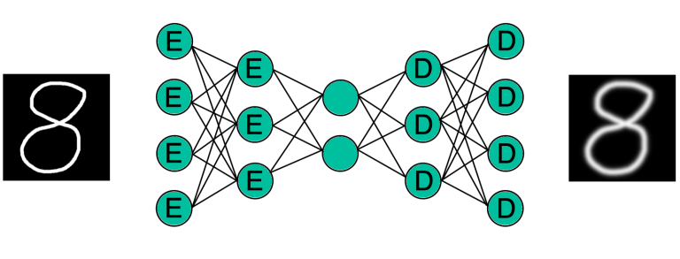
Figure 7 – Autoencoder Example
Once this neural network is built, training is performed by using each image as input and expected output at the same time. Because of its specific design, this network reduces the input image to a simpler representation (sometimes called “compressed”), and then back to the original image. As a result, when the resulting output looks like the input, it means that the information contained in the hidden layer between the “encoder” and the “decoder” should be a good representation of the input image and it could be used in a regular clustering algorithm with success.
Although our original semantic segmented imaged used four different colours (one for each relevant element), to keep this experiment simple, we imported images in grayscale format and their size were also reduced to 512×512 before feeding the neural network. The neural network was designed using a combination of Convolutional Layers and Dense Layers. First, four convolutional and max_pooling layers were used. Then, the result was flattened into an array of 32768 elements, and that was the input of two dense layers that ended with a representation of 128 elements. The details of the neural network can be shown below:
Layer (type)                 Output Shape              Param #
=================================================================
input_1 (InputLayer)         (None, 512, 512, 1)       0
_________________________________________________________________
conv2d_1 (Conv2D)            (None, 512, 512, 16)      160
_________________________________________________________________
max_pooling2d_1 (MaxPooling2 (None, 256, 256, 16)      0
_________________________________________________________________
conv2d_2 (Conv2D)            (None, 256, 256, 8)       1160
_________________________________________________________________
max_pooling2d_2 (MaxPooling2 (None, 128, 128, 8)       0
_________________________________________________________________
conv2d_3 (Conv2D)            (None, 128, 128, 8)       584
_________________________________________________________________
max_pooling2d_3 (MaxPooling2 (None, 64, 64, 8)         0
_________________________________________________________________
conv2d_4 (Conv2D)            (None, 64, 64, 8)         584
_________________________________________________________________
flatten_1 (Flatten)          (None, 32768)             0
_________________________________________________________________
dense_1 (Dense)              (None, 1000)              32769000
_________________________________________________________________
dense_2 (Dense)              (None, 128)               128128
_________________________________________________________________
dense_3 (Dense)              (None, 1000)              129000
_________________________________________________________________
dense_4 (Dense)              (None, 32768)             32800768
_________________________________________________________________
reshape_1 (Reshape)          (None, 64, 64, 8)         0
_________________________________________________________________
conv2d_5 (Conv2D)            (None, 64, 64, 8)         584
_________________________________________________________________
up_sampling2d_1 (UpSampling2 (None, 128, 128, 8)       0
_________________________________________________________________
conv2d_6 (Conv2D)            (None, 128, 128, 16)      1168
_________________________________________________________________
up_sampling2d_2 (UpSampling2 (None, 256, 256, 16)      0
_________________________________________________________________
conv2d_7 (Conv2D)            (None, 256, 256, 16)      2320
_________________________________________________________________
up_sampling2d_3 (UpSampling2 (None, 512, 512, 16)      0
_________________________________________________________________
conv2d_8 (Conv2D)            (None, 512, 512, 1)       145
=================================================================
Total params: 65,833,601
Trainable params: 65,833,601
Non-trainable params: 0
This neural network was trained with the whole dataset during 10 epochs, and the resulting weights were stored for further use. After that, another python script was developed that created a different dataset based on the features obtained from the “encoder” part of the previously mentioned neural network.
Finally, this new dataset was used to feed a K-Means model, obtaining the following results:
| CLUSTER | # ELEMENTS | EXAMPLES |
| 0 | 67 | etsy.com expedia.com kickstarter.com xda-developers.com |
| 1 | 60 | github.com linkedin.com trello.com tumblr.com |
| 2 | 65 | google.* |
| 3 | 112 | bbc.co.uk cbsnews.com cnet.com cnn.com elmundo.es forbes.com foxnews.com |
| 4 | 38 | blogger.com blogspot.* |
| 5 | 48 | akamaihd.net alexa.cn amazonaws.com ask.com bp.blogspot.com |
| 6 | 87 | bbc.com independent.co.uk lequipe.fr marca.com nytimes.com telegraph.co.uk theguardian.com |
| 7 | 61 | alibaba.com amazon.* ebay.* |
| 8 | 146 | aol.com baidu.com google.cn yahoo.com |
| 9 | 64 | answers.com dictionary.com thefreedictionary.com wikipedia.org |
These results showed that some pages covering similar topics were clustered together. Obviously, we were not analysing the content of each website itself, but the design of it in terms of where images, buttons and input boxes are located. However, it is expected that websites covering similar topics also share similar designs and, as a result, their 128-feature vector would be more similar than other websites covering different topics.
An example would be newspapers that were clustered together in cluster 3 and 6, depending on their design, or dictionaries and similar that are clustered in cluster 9. An interesting example is cluster 5, which clusters together a combination of pages that returned an error when they were visited and, therefore, they all look similar to each other.
In summary, we experimented with several approaches to solve this classification problem; the combination of extracting the semantic segmentation of the webpage and using an autoencoder to find a representation of its design was found to be the most promising technique. Further experiments could include using a bigger autoencoder and using the four colours, and not only one of them, and combining this visual design technique with text-based techniques.
